Initial value problem
![\includegraphics[width=5in]{SP3053_figA05_helvetica.eps}](img7.png)
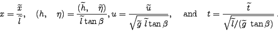
The nonlinear evolution of a wave over a sloping beach is theoretically and numerically challenging due to the moving boundary singularity. Yet, it is important to have a good estimate of the shoreline velocity and associated runup-rundown motion, since they are crucial for the planning of coastal flooding and of coastal structures. As explained in the previous section, Synolakis (1987) solved this problem as a boundary value problem considering canonical bathymetry. Kânoglu (2004) solved nonlinear evolution of any given wave form over a sloping beach as an initial value problem (Fig. 1). It is proposed that any initial waveform can first be represented in the transform space using the linearized form of the Carrier-Greenspan transformation for the spatial variable, then the nonlinear evolutions of these initial waveforms can be directly evaluated. Later, Kânoglu and Synolakis (2006) solved the similar problem considering a more general initial condition, i.e., initial wave with velocity.
Kânoglu (2004) considers NSW equations (![]() ) with
slightly different nondimensionalization than (
) with
slightly different nondimensionalization than (![]() ), i.e.,
using the reference length
), i.e.,
using the reference length ![]() as a scaling parameter,
the dimensionless variables are introduced as
as a scaling parameter,
the dimensionless variables are introduced as
Using the original Carrier-Greenspan transformation--without ![]() coefficient in (
coefficient in (![]() ) and (
) and (![]() )--it is
possible to reduce the NSW equations to the following single
second-order linear equation the same as (
)--it is
possible to reduce the NSW equations to the following single
second-order linear equation the same as (![]() ):
):
using the Riemann invariants of the hyperbolic system (Carrier and
Greenspan, 1958). The Carrier-Greenspan transformation not only
reduces the nonlinear shallow water-wave equations into a
second-order linear equation, but also fixes the instantaneous
shoreline to ![]() in the
in the
![]() -space as
explained previously. Furthermore, a bounded solution at the
shoreline combined with a given initial condition in terms of a wave
profile at
-space as
explained previously. Furthermore, a bounded solution at the
shoreline combined with a given initial condition in terms of a wave
profile at ![]() in the
in the ![]()
![]() -space,
-space,
![]() implies the following solution in the transform space,
implies the following solution in the transform space,

![$\displaystyle -\frac{1}{4}\left\{ \int_{0}^{\infty }\xi ^{2}\Phi (\xi )\left[
\...
...mega \xi )\cos (\omega
\lambda )\mathrm{d}\omega \right] \mathrm{d}\xi \right\}$](img25.png)
![$\displaystyle \mbox{}\!\!\!\!\!\!-\frac{1}{2}\left\{ \int_{0}^{\infty }\xi ^{2}...
...xi
)\sin (\omega \lambda )\mathrm{d}\omega \right] \mathrm{d}\xi \right\} ^{2},$](img26.png)
where, again,
Since it is important for coastal planning, simple expressions for
shoreline runup-rundown motion and velocity are useful. Considering
the shoreline corresponds to ![]() in the
in the ![]()
![]() -space, (4) reduces to the following equation for the
runup-rundown motion:
-space, (4) reduces to the following equation for the
runup-rundown motion:
![$\displaystyle -\frac{1}{4}\left\{ \int_{0}^{\infty }\xi ^{2}\Phi (\xi )\left[
\...
...a \xi )\cos (\omega \lambda )\mathrm{d}\omega %
\right] \mathrm{d}\xi \right\}$](img30.png)
![$\displaystyle \mbox{}\!\!\!\!\!\!-\frac{1}{2}\left\{ \int_{0}^{\infty }\xi ^{2}...
...)\sin (\omega \lambda )%
\mathrm{d}\omega \right] \mathrm{d}\xi \right\} ^{2}.$](img31.png)
Here
The difficulty of deriving an initial condition in the ![]()
![]() -space is overcome by simply using the linearized form of
the hodograph transformation for a spatial variable in the
definition of initial condition. It is proposed that any initial
waveform can first be represented in the transform space using the
linearized form of the Carrier-Greenspan transformation for the
spatial variable ((
-space is overcome by simply using the linearized form of
the hodograph transformation for a spatial variable in the
definition of initial condition. It is proposed that any initial
waveform can first be represented in the transform space using the
linearized form of the Carrier-Greenspan transformation for the
spatial variable ((![]() ) without
) without ![]() coefficient),
then the nonlinear evolutions of these initial waveforms can be
directly evaluated. Once an initial value problem is specified in
the
coefficient),
then the nonlinear evolutions of these initial waveforms can be
directly evaluated. Once an initial value problem is specified in
the ![]() -space as
-space as ![]() , the linearized hodograph
transformation
, the linearized hodograph
transformation
![]() is used directly to
define the initial waveform in the
is used directly to
define the initial waveform in the ![]()
![]() -space,
-space,
![]() . Thus
. Thus
![]()
![]() is found,
and
is found,
and
![]() follows directly through a simple
integration, as in (4). Then it becomes possible to
investigate any realistic initial waveform such as Gaussian and
N-wave shapes employed in Carrier et al. (2003) and the
isosceles and general N-waves defined by Tadepalli and Synolakis
(1994). Again, solution in the physical space can be found using the
Newton-Raphson algorithm proposed by Synolakis (1987) and later
used by Kânoglu (2004), as presented in (A24a, b).
follows directly through a simple
integration, as in (4). Then it becomes possible to
investigate any realistic initial waveform such as Gaussian and
N-wave shapes employed in Carrier et al. (2003) and the
isosceles and general N-waves defined by Tadepalli and Synolakis
(1994). Again, solution in the physical space can be found using the
Newton-Raphson algorithm proposed by Synolakis (1987) and later
used by Kânoglu (2004), as presented in (A24a, b).
The shoreline runup-rundown motion and velocity are presented for
one of the initial profiles given by Carrier et al. (2003):
which leads to the definition of the initial condition
Figure 2a compares the initial waveforms defined
in the physical space as in (6) with the one resulting
from the approximation of it, i.e., (calculated through
(4)). The linearized form of the spatial variable in the
definition of the initial waveforms gives satisfactory comparison.
Figures 2b and 2c present the
shoreline runup-rundown motion and velocity, respectively,
calculated from equation (5) using the corresponding
parts. It should be added that the solution presented here cannot be
evaluated when the Jacobian of the transformation,
![]() , breaks down. Even though
the transformation might become singular at certain points, the
solution can still be obtained at other points, since local
integration can be performed without prior knowledge of the
dependent variables, unlike in numerical methods. This feature is
discussed in detail in Synolakis (1987) and Carrier et al. (2003), and is not explained further in here.
, breaks down. Even though
the transformation might become singular at certain points, the
solution can still be obtained at other points, since local
integration can be performed without prior knowledge of the
dependent variables, unlike in numerical methods. This feature is
discussed in detail in Synolakis (1987) and Carrier et al. (2003), and is not explained further in here.
![\includegraphics[width=5in]{SP3053_figA06_helvetica.eps}](img50.png) |
References:
Carrier, G.F., T.T. Wu, and H. Yeh (2003): Tsunami runup and drawdown on a sloping beach. J. Fluid Mech., 475, 79-99.
Kânoglu, U. (2004): Nonlinear evolution and runup-rundown of long waves over a sloping beach. J. Fluid Mech., 513, 363-372.
Kânoglu, U., and C. Synolakis (2006): Initial value problem
solution of nonlinear shallow water-wave equations. Phys.
Rev. Lett., 97, 148501-148504.